Rapid event-related fMRI studies use closely spaced events leading to
more effective designs than slow event-related paradigms. From the perspective
of the subject, the experiment is also less "boring" than a
slow event-related design which contain long resting gaps between the
events of typically 8-16 seconds. Due to the closely spaced events, the
resulting hemodynamic responses overlap substantially. There are several
important prerequisites in order to be able to analyze rapid event-related
designs: The onsets between successive events must vary (be "jittered)
and a proper balancing of the conditions has to be performed. For details
on rapid event-related fMRI, see Dale & Buckner (199?) etc. Under
the assumption of linearity, the underlying hemodynamic responses might
be estimated by deconvolution.
In principle, rapid event-related paradigms can be analyzed like slow event-related
experiments: Predictors are defined, convolved with the hemodynamic response
function and then subjected to a single or multi-study GLM. In this standard
approach, the hemodynamic response function is fixed.
A deconvolution analysis also consists of a GLM analysis but it estimates
the hemodynamic response function for each event type. In slow event-related
designs, this estimate would correspond to the results of event-related
averaging plots. In rapid designs, the hemodynamic responses have to be
separated and this is done by deconvolution. In the following, the standard
approach to analyze event-related designs is shortly presented followed
by the deconvolution analysis of the same example. The data used here
was kindly provided by Kalanit Grill-Spector (Stanford University). The
preprocessing of (rapid) event-related designs should contain slice time
correction, a high pass temporal filter but no temporal smoothing. The
onsets between events should vary in the range of 2-6 seconds. The validity
of the linearity assumption appears to be decline strongly with delays
shorter than 2-3 seconds. Note that the deconvolution analysis works at
present only for volume-level protocols but not for msec protocols and
only for designs with spaces between events which are multiples of the
TR. A generalization to msec protocols will be implemented in a future
release of BrainVoyager.
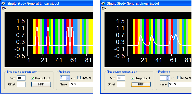
The standard analysis. The figure below shows part of the Single Study General Linear Model dialog with the protocol for the sample data. There are five main conditions (objects presented in various sizes) and one baseline condition (grey color). Predictors for all five conditions have been defined and the figure below shows the time course of predictor 1 (white curve over red conditions) prior (left side) and after (right side) the application of the hemodynamic response function.
The TR of the study was 1 second and the figure on the right shows that
the used hemodynamic response function produces a continous predictor
function shifted appropriately to the right. Note that the onsets between
events were varied at multiples of 3 TRs in this example data, i.e. they
were spaced either by 3 or 6 seconds. The red trials shown shown in the
figure are all defined as 3 second events in the protocol. Note the effect
of the linearity assumption in the predictor function on the right: The
two "red" events on the right side of the graph were spaced
closely leading to a overlapping expected hemodynamic response function.
This model can now be analyzed as usual by clicking the GO
button. In a multi-study
experiment, you would also save the defined single-study design matrices
to disk for each run and use the saved RTC files for a multi-study GLM
analysis (the example actually contains four runs). Having computed the
GLM, you can test contrasts by using the Overlay GLM dialog.
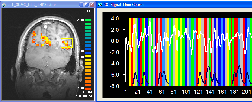
The figure above shows the results of the standard analysis with a time course from a selected ROI on the right. The black curve at the bottom of the graph shows the reference function of the first ("red") predictor. As you can see, the signal follows somewhat this predictor but the respective ROI also responds to other conditions producing a complex response over time. Note that the signal drops nicely after baseline ("grey") conditions.
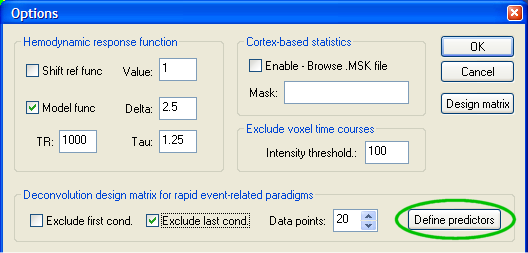
Deconvolution analysis. For the deconvolution analysis, a special design matrix is defined allowing to estimate the response function for each condition. This design matrix could be defined also in previous versions of BrainVoyager but it would consists of a tedious entering process (scripting would be an alternative). An appropriate design matrix can now be defined automatically. After entering the Single Study General Linear Model dialog, click the Options button. In the appearing Options dialog, you will find the HRF deconvolution design for fast event-related paradigms field. Here a set of shifted stick functions can be defined for each event with a single button click. The number of shifted (or delay) predictors is determined in the Data points: box. The default value will define as many shifted predictors as are necessary to "cover" the whole temporal extend of a typical hemodynamic response. The value is internally specified as 20 seconds. Since the TR is 1000 milliseconds, the program recommends to use 20 predictors per event type. Before defining the predictors, you should exclude your baseline condition, which is defined as the last one in the protocol in our example. You can simply click the Define predictors button (see green ellipsoid) to generate the design matrix.
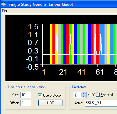
The Single Study General Linear Model dialog will now show 5 x 20 predictors (number of conditions times number of predictors per condition). The figure below shows, for example, predictor 5, which is the stick function for the first condition at delay 4. Note that the names of the predictors (i.e. "SSLS_D4") are constructed automatically by using the condition name "SSLS" plus a "_D<nr>" part reflecting the delay of the function with respect to the begin of the event. These names should not be changed because they are used later for plotting automatically the deconvolved hemodynamic responses.
A more global view on the created design matrix can be obtained by clicking the Design matrix button after reentering the Options dialog. The partial design matrix is shown in the next figure after switching to SPM style and zooming out several times.
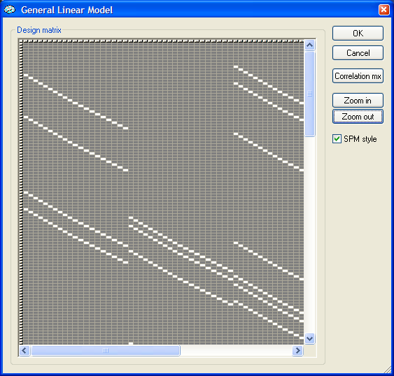
In this graph you can clearly see the shifted stick functions in "packets" of 20 successive columns. You can now run the GLM analysis as usual by clciking the GO button in the GLM dialog. Do not forget to save the created design matrix for each run to allow subsequent multi-study GLM as well as ROI GLM analysis. Since we are going to perform a ROI GLM analysis next, the design matrix has been saved to disk as "sc1.rtc".
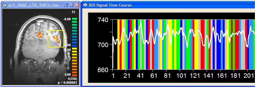
The figure above shows the reulting GLM (full model) and the time course of a selected ROI on the right. To obtain a plot of the deconvolved hemodynamic responses for this ROI, we now perform a ROI GLM analysis. Expand the ROI Signal Time Course window and then click the Options button. In the ROI-GLM field keep the default settings but also check the Correction for serial corr. option. Select the saved deconvolution design matrix file (i.e. "sc1.rtc") using the Browse... button and then click the Fit GLM button. Simply keep all settings in the appearing ROI GLM Specifications dialog and click the OK button. You will now receive the typical ROI GLM output tables and graphs. In addition you will see a new graph showing the deconvolved hemodynamic responses (see figure below).
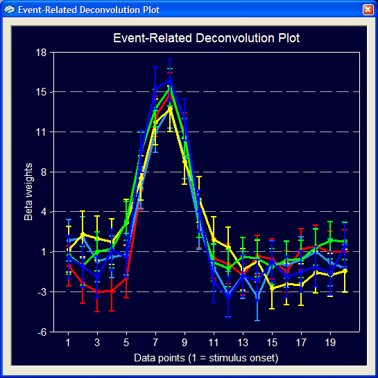
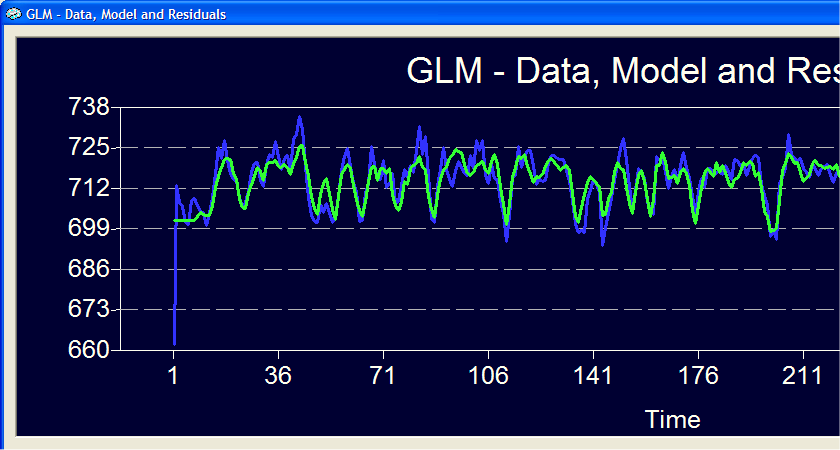
The five curves in this plot reflect the estimated hemodynamic response functions for the five event types. The y axis shows the size of the beta weights and the respective numerical values are also plotted in the tabular output. These estimated functions (and not a fixed predefined HRF) explain the measured time course to a substantial degree as shown in the GLM Data plot (see below). The blue curve is the measured data and the green curve is the fitted signal time course using the estimated hemodynamic response functions shown above (the residuals have been turned off).
Note that the program provides two estimated plots because we have turned on the correction for serial correlations. The standard errors of the second plot might be slightly larger than on the first plot but is the one which should be used for statistical comparisons. Note that you can specify in the ROI GLM Specifications dialog any contrast with the advantage that contrasts can be defined comparing conditions at specific delays. The same holds true for the global overlay GLM function.