Overview. The computation of a single or multi study/subject GLM provides a "GLM" data structure containing for each voxel a set of statistical values including a multiple correlation coefficient and beta weights. These detailed values are not directly accessible for the user, except by reading a saved GLM file. The ROI GLM feature allows to access the statistical parameters for a single voxel. It is, however, not limited to single voxel time courses but computes and displays statistical parameters for the time course of any selected region-of-interest (ROI). The ROI GLM feature also allows to compute and display any set of contrasts. It also allows to correct for serial correlations within the ROI time course presenting all results with properly adjusted parameter values. The application of a ROI GLM will be presented first for the case of a single study, followed by the more general case of multiple studies. The tool works identical for FMR projects and VTC-based projects and is described here in detail only for the latter using data files provided on the BrainVoyager CD.
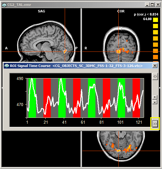
Single study ROI GLM. To access the ROI GLM tool, you must invoke the time course for the desired region-of-interest. For a single study VTC analysis, you must link a VTC file. This is not necessary for FMR projects because the time course data (STC files) is always linked to the FMR project. Now run any of the provided statistical tests to obtain a statistical map. You will later need a single study design matrix (RTC) file. This can be obtained by saving the defined predictors in the Single Study General Linear Model dialog (see Getting Started Guide, tutorial xx or chapter "Design matrix: Construction and visualization"). After running the statistical test, click with the right mouse button on a functional cluster in the VMR window, which will invoke a ROI Signal Time Course window displaying the time course of the selected region-of-interest.
Note: The ROI Analysis tool provides another interesting possibility to obtain a time course for a region-of-interest.

In order to access the ROI GLM feature, "expand" the ROI Signal Time Course window by clicking the Expand button, which is marked in yellow in the figure above. In the expanded window, click the Options button, which will invoke the Options dialog of the ROI Signal Time Course window.

The lower part of the Options dialog contains the ROI-GLM field. The Output subfield contains four general options, from which the GLM graphs and GLM tables options are checked as default. The Auto correlation graphs and Correction for sierial corr. options are not checked as default. We will now keep the default settings but come back later to mark the unchecked options.
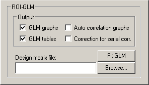
The most important information you have to provide is the design matrix. The specified design matrix is used to analyze the time course of the selected ROI. To select a design matrix file, use the Browse... button next to the Design matrix file: text box. Here we select the "ObjectsDesignMatrix.rtc" file of the "Objects" example.
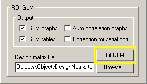
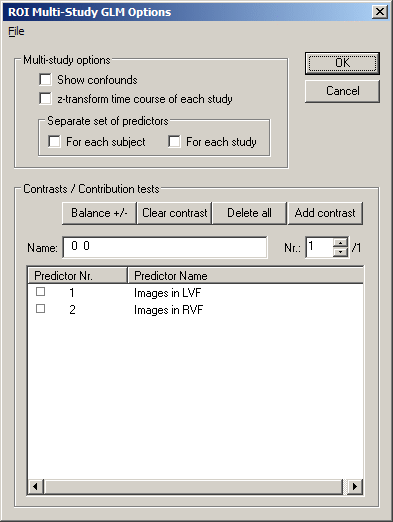
Now we have specified all required information and we can proceed by clicking the Fit GLM button. Before presenting the GLM results, another dialog, the ROI Multi Study GLM Options dialog appears. This dialog lets you specify contrasts in the Contrasts / Contribution tests field as well as further options, which are relevant primarily for multi study design matrices. These options will be described below. For now, we simply click the OK button.
As specified previously (default output options), a GLM graph and a GLM table is presented describing in detail the result of the performed GLM analysis of the selected ROI time course. For our example time course, the GLM graph output is as follows:
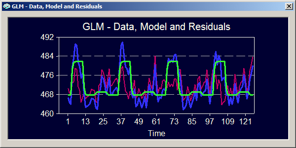
The blue curve represents the data for the GLM, which is the selected ROI time course as also shown in the ROI Signal Time Course window. The green curve represents the model fitted to the data. As you can see, the model nicely reflects the large deflections corresponding to the four "Images in LVF" condition. The pink curve represents the residuals, which are the differences between the data and the model.
NOTE Since the displayed window is a standard plot window like the one used for event-related averaging plots, you can adjust the display using the Plot Options dialog, which can be invoked by simply clicking into the GLM graph window.
Numerical details of the GLM analysis are provided in the GLM table, which is displayed in an HTML window.
NOTE The information is automatically saved to the "ROI_GLM_Info.html" file in the BrainVoyager folder. If you want to save the information from future overwrites, you might want to rename the respective file.
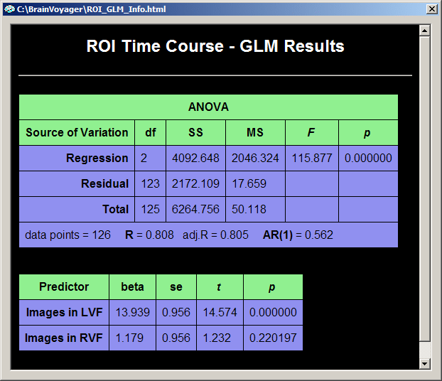
The default output in the GLM table consists of an "ANOVA" table and a "Predictors" table. The ANOVA table shows how the total variance in the data time course (cell "Total - SS", SS = sum of squares) has been divided by the GLM into two parts, the explained variance (cell "Regression - SS") and the unexplained variance (cell "Residual - SS"). The table also shows the degrees of freedom of the total variance (cell "Total - df"), which has been also divided by the GLM into the degrees of freedom for the model (cell "Regression - df")and for the residuals (cell "Residual - df"). The degrees of freedom for the model corresponds to the number of predictors minus 1. Since we have 3 predictors - two main predictors ("Images in LVF", "Images in RVF") plus the constant term predictor, this corresponds to 3 - 1 = 2 degrees of freedom. The values of the column "MS" (mean squares) are obtained by dividing the respective sum of squares by the respective degrees of freedom: MS = SS / df. The obtained MS values for the model ("Regression") and residuals are used to compute an F statistic, which assesses the goodness-of-fit of the model: F = MSRegression / MSResidual. Together with the degrees of freedom for the model and the residuals, this F value corresponds to a p-value assessing the significance of the model fit. In the bottom row, the ANOVA table also shows the number of data points and the multiple correlation coefficient R as well as an adjusted version. The multiple correlation coefficient also assesses the goodness-of-fit being the square root of the ratio of explained to total variance: R2 = (explained variance) / (total variance) = SSRegression / SSTotal. The last value in the bottom row of the ANOVA table, "AR(1)" (lag 1 auto-regression) assesses serial correlations within the ROI time course (see section "Serial correlations" for details).
The "Predictors" table contains one row for each main predictor of the model. The first column contains the names of the predictors, in our case "Images in LVF" and "Images in RVF". The second column contains the beta weights for each predictor. In combination with significance values, these beta weights are the most important result of a GLM analysis and are estimated to fit the specified model as good as possible (in the least squares sense) to the data. The model, the green curve in the GLM output graph, is computed by multiplying the model function for each predictor with the respective beta weight and summing the obtained values for each data point. Therefore the green curve shows high values (beta weight:13.939) in the four segments corresponding to the first predictor ("Images in LVF") and low values (beta weight: 1.179) for the four segments corresponding to the second predictor ("Images in RVF"). There are three more columns assessing the significance of the beta weights, the "se" columns containing the standard errors of the beta weights, the "t" column and the "p" column.
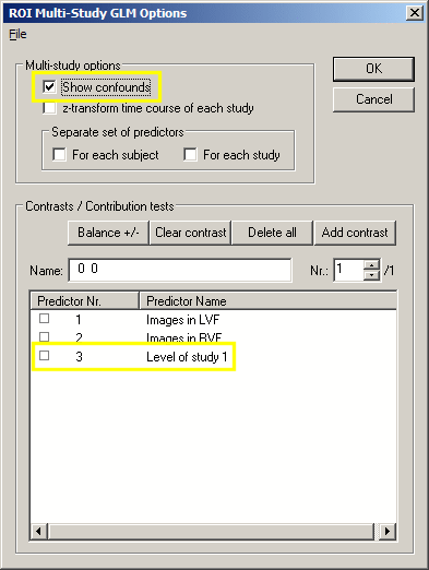
There is one predictor missing in the table, the "confound" predictor with the value "1" for each data point. This "constant term" predictor is used to fit the overall signal level of the time course. To see this predictor, close the GLM output windows. In the ROI Signal Time Course window, click the Options button and in the appearing Options dialog, click the Fit GLM button. If you now check the Show confounds option in the ROI Multi Study GLM Options dialog, the constant term predictor automatically appears in the Predictors list box named as "Level of study 1":
If you now click the OK button, the GLM table output is identical as before except that the constant term predictor has been added:
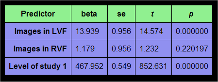
With the complete set of beta weights, the model value for each data point can now precisely computed as the sum of the "beta weight x predictor value at data point" products.
Besides the ANOVA table and the Predictors table described above, the tabular GLM output will also show numerical details for specified contrasts. Since we have not yet specified any contrast, this table does not appear in the output window. To define contrasts, close the output windows. In the ROI Signal Time Course window, click the Options button and in the appearing Options dialog, click the Fit GLM button. Now define contrasts by "+" and "-" checking of the listed predictors. As an example, we will define three contrasts. For the first contrast, set the first predictor, "Images in LVF" to "+". Add another contrast by clicking the Add contrast button. Now set the second predictor, "Images in RVF" to "+", which defines the second contrast. Click again the Add contrast button to define the third contrast. This contrast should compare the two predictors, thus, set the first predictor to "+" and the second predictor to "-" as shown below:
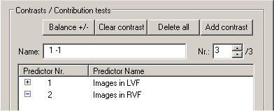
The Nr.: text box shows that we have selected the third contrast from the overall set of three predictors (indicated by "/3" on the right side of the Nr.: text box). The selected third contrast is shown in the left column of the Predictors list box and its name is shown in the Name: text box. The name of a contrast reflects the "+" and "-" selections with integral values (i.e. "1", "-1") as default. You can, however, change it to any string. There are additional buttons helping you to define contrasts. The Delete all button removes all defined contrasts. The Clear contrast button clears the "+" / "-" settings in the left column of the Predictors list box. The Balance +/- button can be used to equalize the sum of all positive entries with the sum of all negative values, which is recommended for any contrast. By <Shift>-clicking on a square in the left column of the Predictors list box, you can enter any integral value for the respective contrast element (predictor).
After clicking the OK button in the ROI Multi Study GLM Options dialog, the tabular output now contains two further tables, one for all defined contrasts ("Contrasts/LF" table) and one with a contribution analysis ("Source of variation" table). The latter table only appears for those contrasts which contain only positive and zero values.
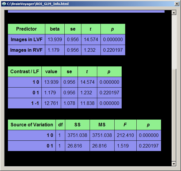
The individual contrasts are identified in the contrast table by their names. A name like "1 -1" corresponds to a contrast where predictor one ("Images in LVF") has been "+" selected and predictor two ("Images in RVF") has been "-" selected. Each row presents numerical information for one contrast. From the information provided, the most important one are the "t" and "p" columns assessing the significance of a contrast.
The "Source of Variation" table analyzes the proportion of variance contributed by a subset of predictors. This is done by performing a model comparison: the full model containing all predictors is compared with a restricted model containing all predictors but those which are "+" selected, i.e. contain a "1". in the contrast name. The question answered here is: Given the restricted model, what is the contributed or additionally "explained" variance of the "1" predictors? The set of plus-predictors can be any number of predictors and mathematically requires an F test (see "F" column) to assess a significant contribution. In our example, two model tests are performed, each having only one "1" predictor. In this case the F test corresponds to the square of the t test for that predictor. The first model test ("1 0"), for example, has an F value of "212.41" which is the square of "14.574", the t value of the "1 0" contrast and the t value for the beta weight of the first predictor ("Images in LVF").
Another option of the ROI GLM feature is the analysis and correction of serial correlations in the ROI time course. This feature is not turned on as default. To enable this feature, close all GLM output windows. In the ROI Signal Time Course window, click the Options button and in the appearing Options dialog, check the Auto correlation graphs and Correction for serial corr. options as shown below:
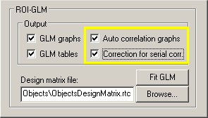
Now click the Fit GLM button and then the OK button in the ROI Multi Study GLM Options dialog. The program now presents several graphs, which will be described shortly. In addition, the numerical output window will now present all tables twice, first without the correction of detected serial correlations ans second, with the correction of serial correlations. The first set of tables is identical to the ones described above. The second set of tables starts with the text line "After correction of serial correlations:" as shown below:
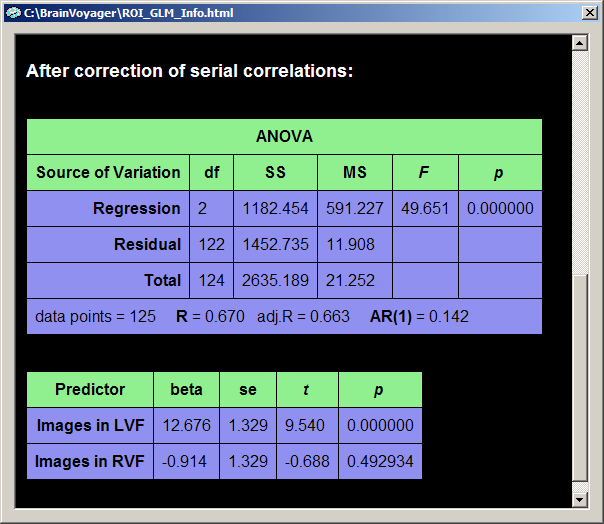
The ROI time course has indeed high serial correlations as assessed by the one-lag auto-correlation term (AR(1) = 0.562). After the correction of serial correlations, the one-lag auto-correlation term is only AR(1) = 0.142. After removing the serial correlations, the program recomputes all statistical values. As you can see, the beta weights have similar values afterwards. The correction of serial correlations does not change the beta weights dramatically (the fitted model is roughly the same), but it might substantially reduce the statistical significance of the beta weights, predictors and contrasts. This can also be seen from the multiple correlation coefficient which is now R = 0.670 but was "0.808" prior to correction of serial correlations.
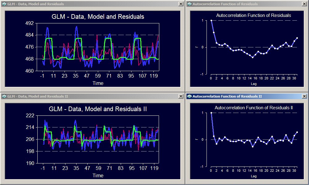
In addition to the numerical, tabular output, you will also obtain graphical output (if chosen), which shows in the upper left window the original time course with the fitted GLM model and the residuals ("GLM - Data, Model and Residuals"), and in the lower left window the corrected time course with the fitted GLM model and residuals. On the right side, two graphs present the autocorrelation function of the residuals before (upper window) and after (lower window) correction of serial correlations. These graphs shows autocorrelation values with respect to "lag" values. These lag values specify correlations of a time course with a shifted version of itself. A lag value of "0" means that the time course has been correlated with an identical copy and, thus, the autocorrelation must be "1". A lag value of "1" means that a copy of the time course is made, which is then shifted one measurement (data point) to the right prior to computing the correlation. The resulting correlation value is the second plotted point in the respective graphs. As you can see, the lag-1 autocorrelation is high in the upper panel, but low in the second panel. The exact numerical values of the lag-1 autocorrelation can be found in the tabular output window ("AR(1)"). For the correction of serial correlations, only the lag-1 autocorrelation is used. The autocorrelation values for further lags are shown for informative purposes only.
Multi study ROI GLM. The ROI GLM feature can be applied to complex design matrices referring to many studies. You can perform for a ROI the same kind of analysis as those you can do in the General Linear Model: Multi Study, Multi Subject dialog. The only difference to the description above is that you have to specify a multi study design matrix definition (MDM) file. The chapter "Design matrix: Construction and visualization" describes in detail how to create multi study design matrices and how to save corresponding MDM files. In the following, data from the "ClockTask" folder is used to describe those options which are particularly relevant for multi study GLMs, all other features (i.e. correction for serial correlations) work identical as described above for single study analyses. The "ClockTask" folder is located in the "Samples" directory of the BrainVoyager CD; it might be also in your BrainVoyager folder of your hard disk (i.e. "C:\Program Files\BrainVoyager\Samples\ClockTask") in case you have chosen to install this data during program installation.
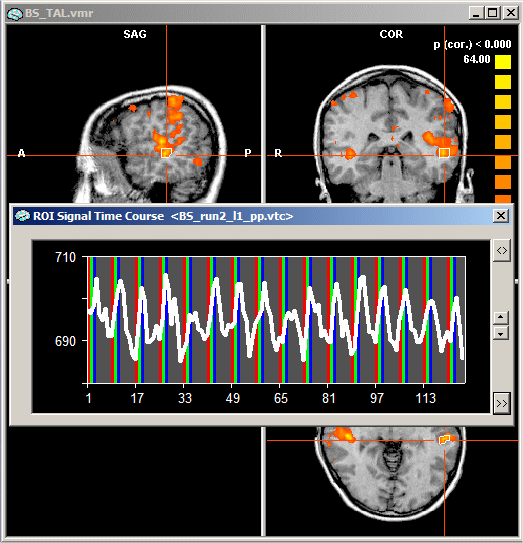
As with single study ROI GLM analysis, the first thing you must do is to select a region-of-interest. This was done for the following figure by opening the "BS_TAL.vmr" file in the "ClockTask" folder, entering the Overlay GLM Contrasts and Contribution Maps dialog, loading the "ClockTask.glm" file, clicking the Fill contrast button and then the OK button. In the displayed map, a region in the auditory cortex has been selected with standard left mouse navigation and then a click with the right mouse button was done to define the ROI and to obtain a ROI Signal Time Course window.
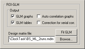
In order to access the ROI GLM feature, "expand" the ROI Signal Time Course window by clicking the Expand button as described above. In the expanded window, click the Options button, which will invoke the Options dialog of the ROI Signal Time Course window. The lower part of the Options dialog contains the ROI-GLM field. As before, the most important information you have to provide is the design matrix. The specified design matrix is used to analyze the time course of the selected ROI. To select a design matrix file, use the Browse... button next to the Design matrix file: text box. Here we select the "BS_ML_2runs.mdm" file located in the "ClockTask" folder.
An MDM file does contain a list of pairs, each pair referring to a time course file (VTC or FMR) and a single study design matrix file. This means that the time course you see in the ROI Signal Time Course window will not necessarily be analyzed. For a multi study analysis, only the defined ROI is used all further information, time course files and single study design matrices, are used as specified in the MDM file (for details, see chapter "Design matrix: Construction and visualization").
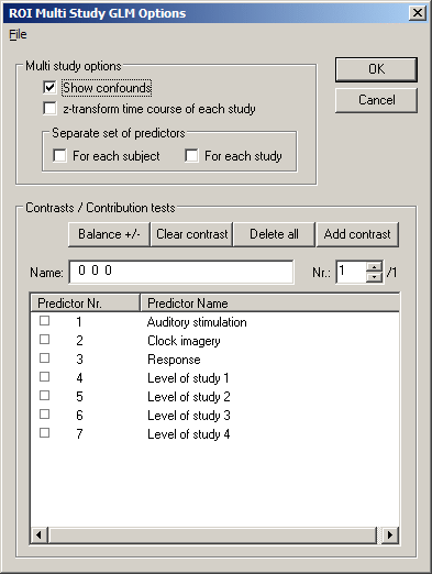
After having specified the multi study design matrix definition file, click the Fit GLM button, which will invoke the ROI Multi Study GLM Options dialog. In the Multi study options field, check the Show confounds option, which will show the four constant term predictors estimating the signal levels for the four studies referenced by the MDM file. We will come back to enable other options, but now proceed by clicking the OK button.
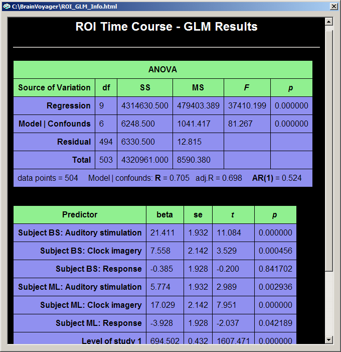
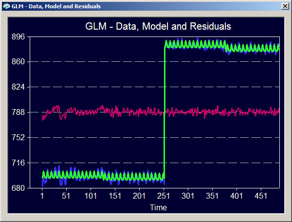
The graphical output shows that the time courses from the four referenced VTC files are concatenated to form the time course for the GLM analysis (4 x 126 = 504 data points). You also see that the first two studies from subject "BS" and the last two studies from subject "ML" have very different signal levels. But also the two studies from the same subject have slightly different signal levels although they were recorded in two successive runs in a single scanning session. This clearly shows that the constant term predictors are necessary to "explain" the variance due to these signal level differences.
The tabular output shows two rows in the ANOVA table to differentiate between the explained variance of the model with all predictors (constant term predictors plus main predictors in the "Regression" row) and the explained variance of the model when the explained variance due to the different signal levels has been removed ("Model | Confounds" row). The latter source of variance is compared to the "total | confounds" variance remaining after the variance explained by the confounds has been subtracted from the total variance. The remaining total variance "total | confounds" can be computed from the table as the sum of the "Model | Confounds" and the "Residual" sum-of-squares. The multiple regression coefficient is then computed as R2 = SSModel | Confounds / ( SSModel | Confounds + SSResidual ).
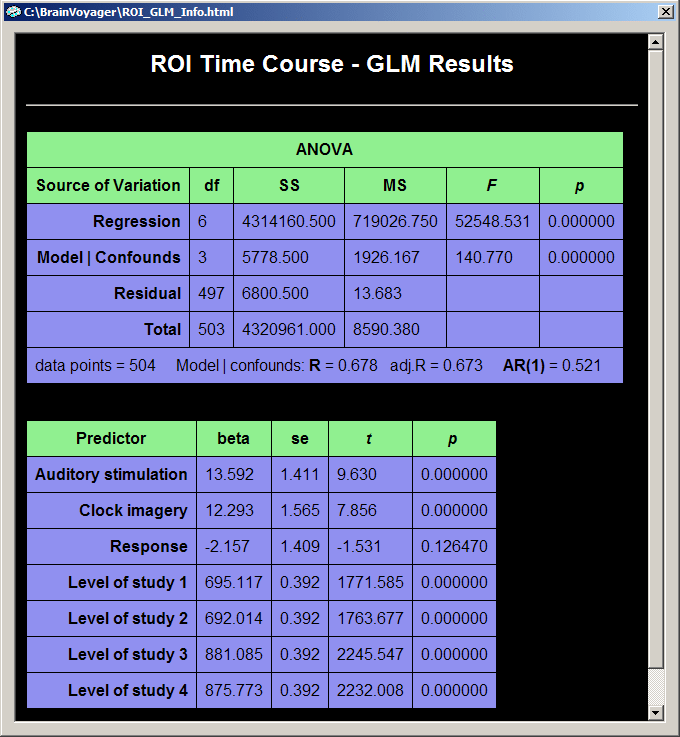
The beta weights of the Predictor table show numerically the observed differences in mean signal intensity of the four studies (last four rows). The first three rows show the beta weights of the three main predictors "Auditory stimulation", "Clock imagery" and "Response". Since we have neither specified "separate study predictors" nor "separate subject predictors", there is only one set of beta weights available to fit the data across all four studies.
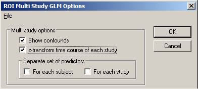
To explore further multi study GLM options, close all output windows and reenter the ROI Multi Study GLM Options dialog. In addition to the Show confounds option, check also the z-transform time course of each study option, then click the OK button.
The graphical output now shows that the signal levels have been equalized due to the z-transformation. A z-transformation removes the mean signal level from each study (i.e. the new mean is "0") and scales the data in such a way that the new standard deviation is "1" ( z = (y - mean_y) / sigma_y ).
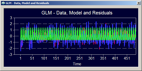
Because of equal signal levels of each study, the sum-of-squares for the "Regression" and "Model | Confounds" components are identical in the ANOVA table in contrast to the previous analysis. The multiple correlation coefficient is not exactly the same as before because the z-transformation not only equalizes the signal level but also the standard deviations of the included studies. This means that each study can contribute equally to the estimation of the model parameters.
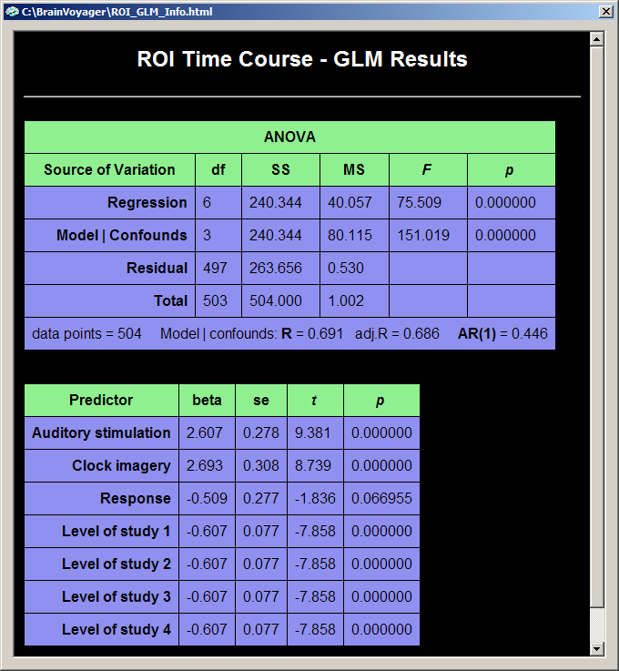
The predictors show a similar pattern as before but are much smaller now due to the z-transformation. The confound predictors for the signal levels are not zero because they do not estimate the study means (which are zero), but the signal levels in the baseline episodes.
We still have one predictor set fitted to the time course comprised of all four studies. There are two other ways to specify beta weights, namely a separate set for each subject or a separate set for each study. The latter case produces more sets of predictors than the first if each subject contributes with more than one study. To specify these options, close all output windows and reenter the ROI Multi Study GLM Options dialog. In addition to the Show confounds option, check the For each subject option (or For each study option) in the Separate set of predictors field. The Predictors list box in the Contrasts / Contribution tests field immediately reflects the made setting by adding (or removing) the respective sets of predictors for each subject (or study). Now click the OK button.
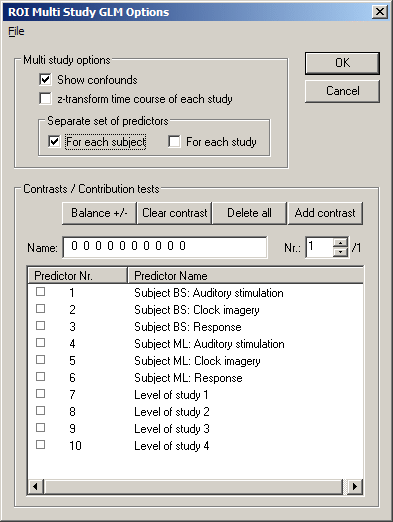
The tabular output shows that the multiple regression coefficient is slightly higher with two predictor sets, one for each subject, than in the case of a single set of beta weights. The reason for this is that the predictors can be adapted optimally for the time course from each subject.
