
Introduction. The General Linear Model is used as the main hypothesis-driven analysis tool in BrainVoyager. For its proper application, several prerequisites have to be fulfilled for each voxel time course the GLM is applied to. One of these prerequisites states that the residuals of any pair of data points within a voxel time course have to be uncorrelated. Residuals are obtained after subtracting the fitted model from the actual voxel time course. For any voxel or ROI time course, the fitted GLM, the actual data and the residuals can be visualized with the ROI-GLM tool. In the case of measuring a phantom or at brain regions not "interested" in any condition of a stimulation protocol, the actual time course of a voxel corresponds to the residuals since a GLM will only fit a constant term for the signal level. Since fMRI data is acquired sequentially, the measurement hardware appears to introduce serial correlations between neighboring measurement time points. These serial correlations are typically positive which means that a positive residual (a value above the mean signal level) will be followed more likely by another positive residual than a negative one and a negative residual (a value below the mean signal level) will be followed more likely by another negative value.
Effects of serial correlations on a GLM. If serial correlations do occur and if this violates one assumption of the GLM, is it then "allowed" to run a GLM at all? It can be shown that the fitted model (the set of beta weights) estimated is approximately the same with or without serial correlations in the residuals. The GLM appears, thus, to be robust against the violation of this assumption. However, the statistical significance of the overall model, and of each of its beta weights, is overestimated ("too good") in the presence of serial correlations. This means that the values of the resulting beta weights are estimated correctly but their standard errors are estimated wrongly, i.e. smaller than they should be. The net result is that you get contrasts more easily "significant" than it should be.
Correcting for serial correlations. You can visualize and correct serial correlations for any ROI time course, for details, see chapter "ROI GLM: Detailed analysis for regions-of-interest". In addition, you can correct for serial correlations while computing a General Linear Model. Invoke the General Linear Model: Multi Study, Multi Subject dialog by selecting the Analysis -> General Linear Model: Multi study... menu item. Define or load a multi study design matrix as described in chapter "Design matrix: Construction and visualization". Note that you can also analyze a single study using the multi study GLM dialog. Now click the Options button, which will invoke the Multi Study GLM Options dialog.
In the Serial correlation of residuals
field, you will find three check boxes. Check the first option, Remove AR(1) and refit GLM to remove
serial correlations. With this option checked, each voxel time course
is analyzed twice. In the first
analysis, a GLM is fitted without considering serial correlations. This
first fit provides residuals by subracting the model from the data. These
residuals are analyzed for serial correlations by computing the one-lag
auto-correlation (AR(1)). The time course is then adjusted based on this
analysis to remove the detected serial correlations. Then this time course
is used to fit the final GLM to the data.
The two other options are only for visualization purposed allowing to visualize
the computed AR(1) term at each voxel in a generated 3D map (VMP) data
structure. You can also visualize the AR(1) terms after removal to verify
the successful operation of the procedure.
Check all three options and run the GLM. The overall model and any defined contrast will produce less activated voxels than without the correction for serial correlations given the same threshold. In addition to producing the corrected GLM, you will also find two VMP files in the current folder, "PreAR1.vmp" and "PostAR1.vmp". You can load these files in the Overlay Statistical Maps dialogs, which is invoked by clicking the Analysis->Overlay maps... menu item. In the dialog's local file menu, use the Load 3D map... menu item and select one of the two VMP maps and then click the Open button.

Now click the OK button In the Overlay Statistical Maps dialog. The following figure shows the "PreAR1.vmp" map for the "Objects" example:
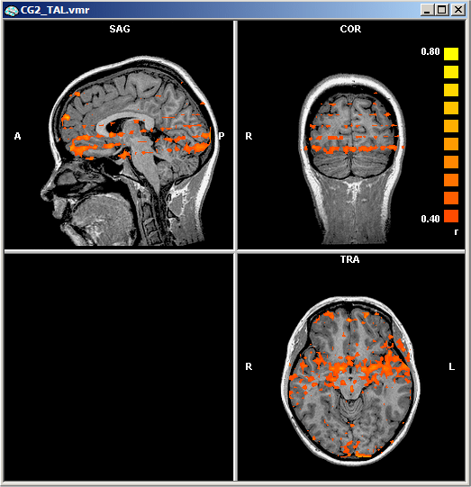
The correlation threshold (AR(1) threshold) is set to 0.4 in the figure above showing substantial serial correlations in some regions of the brain. The respective AR(1) map after correction of serial correlations ("PostAR1.vmp") is shown next:

Note that the threshold has been lowered substantially (0.16) but there are still only a few brain regions color-coded demonstrating a successful correction for serial correlations. For further details, see chapter "ROI GLM: Detailed analysis for regions-of-interest".